African Mammals

Last updated on Jan 12, 2020 10 min read

Interested in the distribution of animal species on a global or continental level? This can be easily illustrated with R using the data provided by the IUCN Red List. In this post, I will focus on mammals in Africa, the continent where I have conducted most of my field work. But the code below can be easily adapted to other areas of the world and other taxonomic groups of species, or only species at low or high risk of extinction (though the completeness of the IUCN data is variable across different groups).

In this post, I describe the following steps:

Download and process the IUCN Red List spatial data set for terrestrial mammals
Download a map of Africa
Create a hexagon grid for Africa
Combine species ranges with the grid and plot the map

The processing and summarizing of the spatial data is mostly done with the impressive sf package. For my first attempts to work with spatial data in R (more specifically with vector data), I used the sp package. But the sf package, which is the successor of the sp, is much easier to use. Additionally, it integrates some of the tidyverse functions, most importantly many of the dplyr functions, which so many R users are already using for other purposes. Also, the sf package is very well documented and the vignettes are extremely helpful. They can be found on the github page of the package or by typing vignette(package = "sf"). I also would like to mention the book ‘Geocomputation with R’, which is a very informative (open source) resource for anybody interested in working with spatial data in R.

1. Download and process the IUCN Red List spatial data set for terrestrial mammals

1.1 Prepare R

rm(list = ls())
library(tidyverse)
library(sf)

1.2 Download and process the IUCN terrestial mammals shapefile

The IUCN Red List spatial data can be obtained here. The IUCN datasets are freely available for non-commercial use, but they have to be downloaded manually because you have to register for an account and provide a description of the intended usage. For academic use, you can (usually) download the dataset immediately after you made your request.

The ranges of populations and species are all provided as polygons in the downloadable shapefiles. However, some species might be missing, and some ranges might be incomplete. Nevertheless, it is an impressive data set, and at least for primates, it looks fairly complete. Further details (and limitations) can be found on the IUCN spatial data webpage.

For this post, I downloaded the “Terrestrial Mammal” datasets, which is about ~ 600 MB. Then, I moved the downloaded folder (‘TERRESTRIAL_MAMMALS’) into the folder “~/Sync/iucn_data/” on my harddrive and renamed it to ‘TERRESTRIAL_MAMMALS_2020_01_11’.

I split up the following process into two steps: 1) load, simplify (i.e., reduce the size of the object), and save the processed shapefile a .gpkg file; and 2) re-load the processed files. The first step will not be evaluated in the final notebook so that the 600 MB shapefile does not have to be processed every time I run this notebook.

mammals <- st_read("~/Sync/iucn_data/TERRESTRIAL_MAMMALS_2020_01_11")

# Simplify the polygons to reduce the size of the object/file. This may take a
# few moments but the size of the object (in the R environment) changes from 906
# Mb to <10 Mb (with dTolerance = 5), which is much easier to handle.
mammals_simple <- mammals %>% 
  st_simplify(dTolerance = 1)

mammals_simple <- mammals_simple %>% 
  select(binomial, presence,legend, category)

# Write the object to a file and clean up. I use .gpkg extension here because it
# just requires one file instead of several files created for shapefiles. Also,
# it's an open format and it appears to be just as good as shapefiles (at least
# for everything I've done so far). Look here for more information:
# https://www.gis-blog.com/geopackage-vs-shapefile/
file_name <- paste0(dirname(here::here()), "/blog_data/iucn_mammal_distribution.gpkg")
st_write(mammals_simple, file_name)
rm(list = c("mammals", "mammals_simple", "file_name"))

Note: I set the dTolerance argument to 1, but for a more precise map, it might be good to change it to 0.1 or a lower value.
Also, I only kept four of the columns: binomial (the species name), presence and legend (indicating whether a population is still present), and category (the risk category for each species). For other projects, additional columns can be added. For example, order_ or family indicate the taxonomic order/family of a species.

Now, load the file (step 2)

file_name <- paste0(dirname(here::here()),
                    "/blog_data/iucn_mammal_distribution.gpkg")
mammals <- st_read(file_name)

## Reading layer `iucn_mammal_distribution' from data source `/Users/urs/Google Drive/Data Blog/blog_data/iucn_mammal_distribution.gpkg' using driver `GPKG'
## Simple feature collection with 12908 features and 4 fields (with 7579 geometries empty)
## geometry type:  MULTIPOLYGON
## dimension:      XY
## bbox:           xmin: -179.999 ymin: -56.04993 xmax: 179.999 ymax: 89.9
## epsg (SRID):    4326
## proj4string:    +proj=longlat +datum=WGS84 +no_defs

Quick look at the sf object:

head(mammals)

## Simple feature collection with 6 features and 4 fields (with 2 geometries empty)
## geometry type:  MULTIPOLYGON
## dimension:      XY
## bbox:           xmin: -58.02031 ymin: -43.29721 xmax: 153.0728 ymax: 50.38943
## epsg (SRID):    4326
## proj4string:    +proj=longlat +datum=WGS84 +no_defs
##                   binomial presence            legend category
## 1 Nyctereutes procyonoides        1 Extant (resident)       LC
## 2         Rattus lutreolus        1 Extant (resident)       LC
## 3     Rhinolophus subrufus        1 Extant (resident)       DD
## 4           Mops spurrelli        1 Extant (resident)       LC
## 5         Clyomys laticeps        1 Extant (resident)       LC
## 6       Eonycteris spelaea        1 Extant (resident)       LC
##                             geom
## 1 MULTIPOLYGON (((143.7874 50...
## 2 MULTIPOLYGON (((147.0231 -3...
## 3             MULTIPOLYGON EMPTY
## 4 MULTIPOLYGON (((16.12875 4....
## 5 MULTIPOLYGON (((-47.53412 -...
## 6             MULTIPOLYGON EMPTY

For an explanation of sf objects, look at the first vignette of the sf package. Every row in this data frame represents one population of species binomial, with additional information about the presence and risk category (columns presence, legend, and category). The sf-column geom contains the geographic information describing the range of each population. As far as I understand this data set, several populations might be combined into one row (the sf-column can contain several polygons), but in other cases, each population has its own row.

We can simply plot all polygons (for all rows) with:

{
  par(mar = c(0, 0, 0, 0))
  plot(st_geometry(mammals))
}

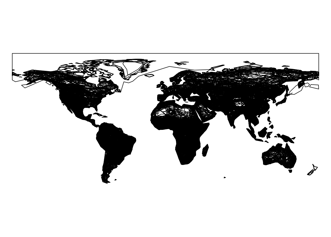
This plot shows the distributions of all mammal species/populations, but it also includes populations that are no longer present. Let’s have a look at the different codes for presence and the description, which can be found in the column legend.

mammals %>%
  st_set_geometry(NULL) %>%
  distinct(presence, legend) %>% 
  arrange(presence)

##    presence                                            legend
## 1         1                                 Extant (resident)
## 2         1                    Extant & Introduced (resident)
## 3         1                  Extant & Reintroduced (resident)
## 4         1          Extant & Vagrant (seasonality uncertain)
## 5         1              Extant & Origin Uncertain (resident)
## 6         1                    Extant (seasonality uncertain)
## 7         1                             Extant (non-breeding)
## 8         1                       Extant & Vagrant (resident)
## 9         2                        Probably Extant (resident)
## 10        2     Probably Extant & Origin Uncertain (resident)
## 11        2           Probably Extant & Introduced (resident)
## 12        3                        Possibly Extant (resident)
## 13        3     Possibly Extant & Origin Uncertain (resident)
## 14        3           Possibly Extant (seasonality uncertain)
## 15        3                         Possibly Extant (passage)
## 16        3 Possibly Extant & Vagrant (seasonality uncertain)
## 17        3           Possibly Extant & Introduced (resident)
## 18        3          Possibly Extant & Vagrant (non-breeding)
## 19        4                                  Possibly Extinct
## 20        4                     Possibly Extinct & Introduced
## 21        5                                           Extinct
## 22        5                        Extinct & Origin Uncertain
## 23        5                              Extinct & Introduced
## 24        5                            Extinct & Reintroduced
## 25        6                                Presence Uncertain
## 26        6             Presence Uncertain & Origin Uncertain
## 27        6                      Presence Uncertain & Vagrant

Codes/numbers 1, 2, and 3 refer to ‘extant’, ‘probably extant’, and ‘possibly extant’ populations, and I only keep these populations here.

mammals_extant <- mammals %>% 
  filter(presence %in% c(1,2,3))

2. Download a map of Africa

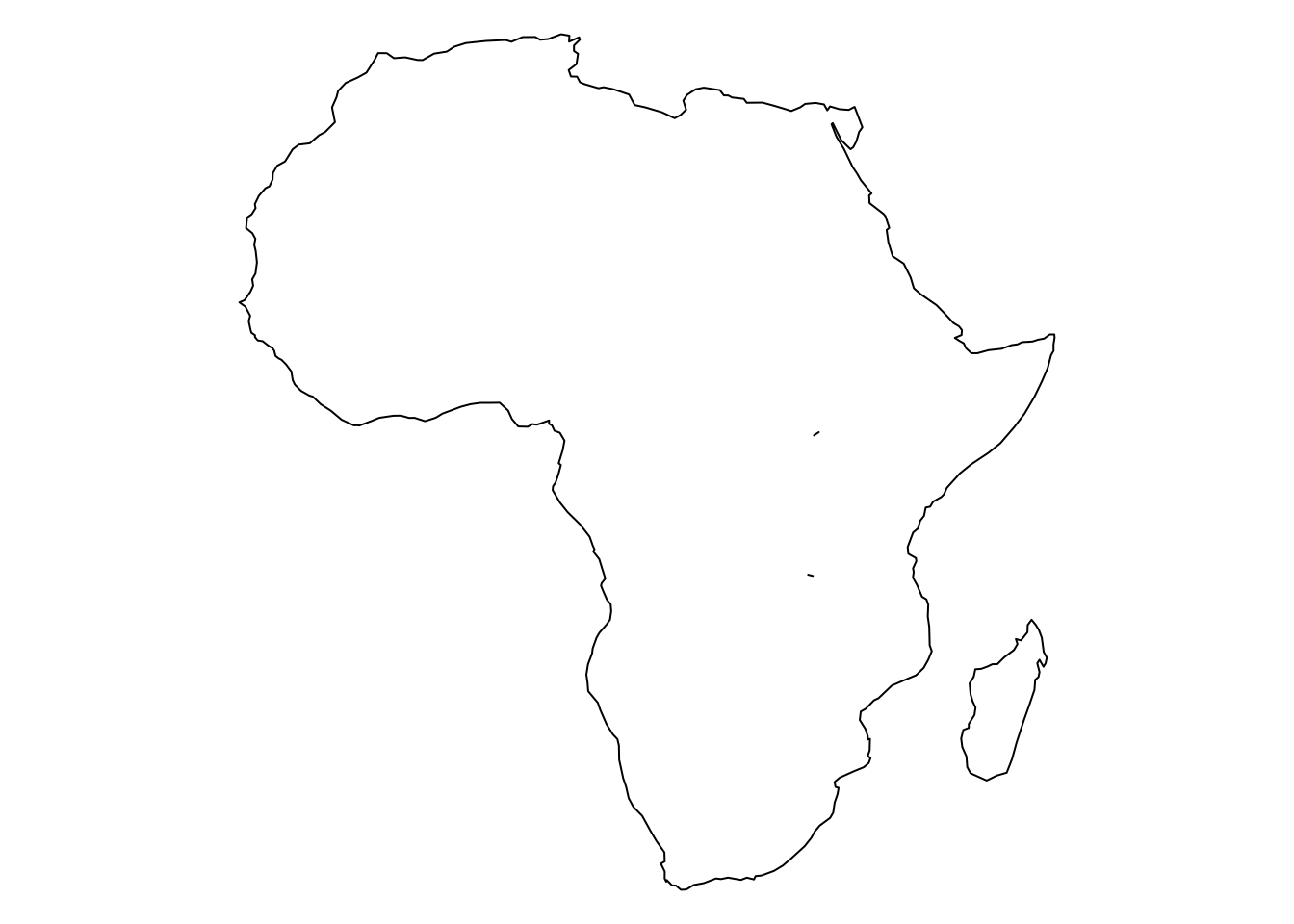
In R, it’s very easy to get maps of countries or continents from https://www.naturalearthdata.com using the rnaturalearth package. With the ne_countries() function, all countries (as polygons) for the specified continent can be downloaded. Here, I am only interested in a map of the whole continent, not single countries. This can be achieved with the dplyr::summarize() function, which ‘summarizes’ the polygons in all rows in the sf object (the countries) to one polygon (the continent). One of the examples showing how nicely the tidyverse functionality is integrated into the sf package!

africa_map <- rnaturalearth::ne_countries(continent = "Africa",
                                          returnclass = "sf") %>%
  st_set_precision(1e9) %>%
  summarize
{
  par(mar = c(0, 0, 0, 0))
  plot(st_geometry(africa_map))
}

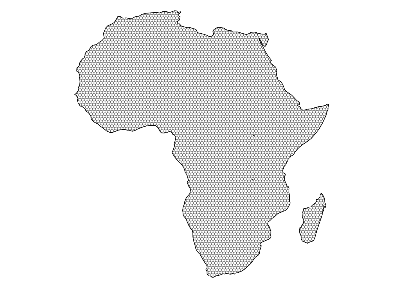
3. Create a hexagon grid for Africa

Since I want to illustrate how species richness varies across regions, the number of species have to be summarized for some kind of (spatial) subsets of Africa. For example, this could be done by country. But here, I use a grid of equally sized hexagon cells to illustrate the varying species richness across the continent. This is possible with the sf::st_make_grid() function. The argument square = F specifies that hexagons are created instead of squares. Furthermore, I create a grid_id column, which will be required as identifier for grid cells further below.

africa_grid <- st_make_grid(africa_map,
                            what = "polygons",
                            cellsize = 0.75,
                            square = F) %>% 
  st_sf() %>% 
  mutate(grid_id = row_number())

Note: the cell size can be adjusted by changing the cellsize argument, but this will also affect the number of species per cell. Larger cells are more likely to intersect with more species than smaller cells.

For the map, I only want to keep the parts of the grid cells that are on the continent. This might be problematic in some cases because the cells at the edge of the continent are smaller than cells within the continent. But since I only summarize terrestrial mammals here, I think it might also be misleading if the cells cover non-terrestrial area without including marine mammals.

africa_grid_clipped <- st_intersection(africa_grid, africa_map)

{
  par(mar = c(0, 0, 0, 0))
  plot(africa_map$geometry, reset = F, axes = F)
  plot(st_geometry(africa_grid_clipped), color = "white",
       add = T, border = rgb(0, 0, 0, 0.3))
}

4. Combine species ranges with the grid and plot the map

4.1 Only keep population ranges within Africa

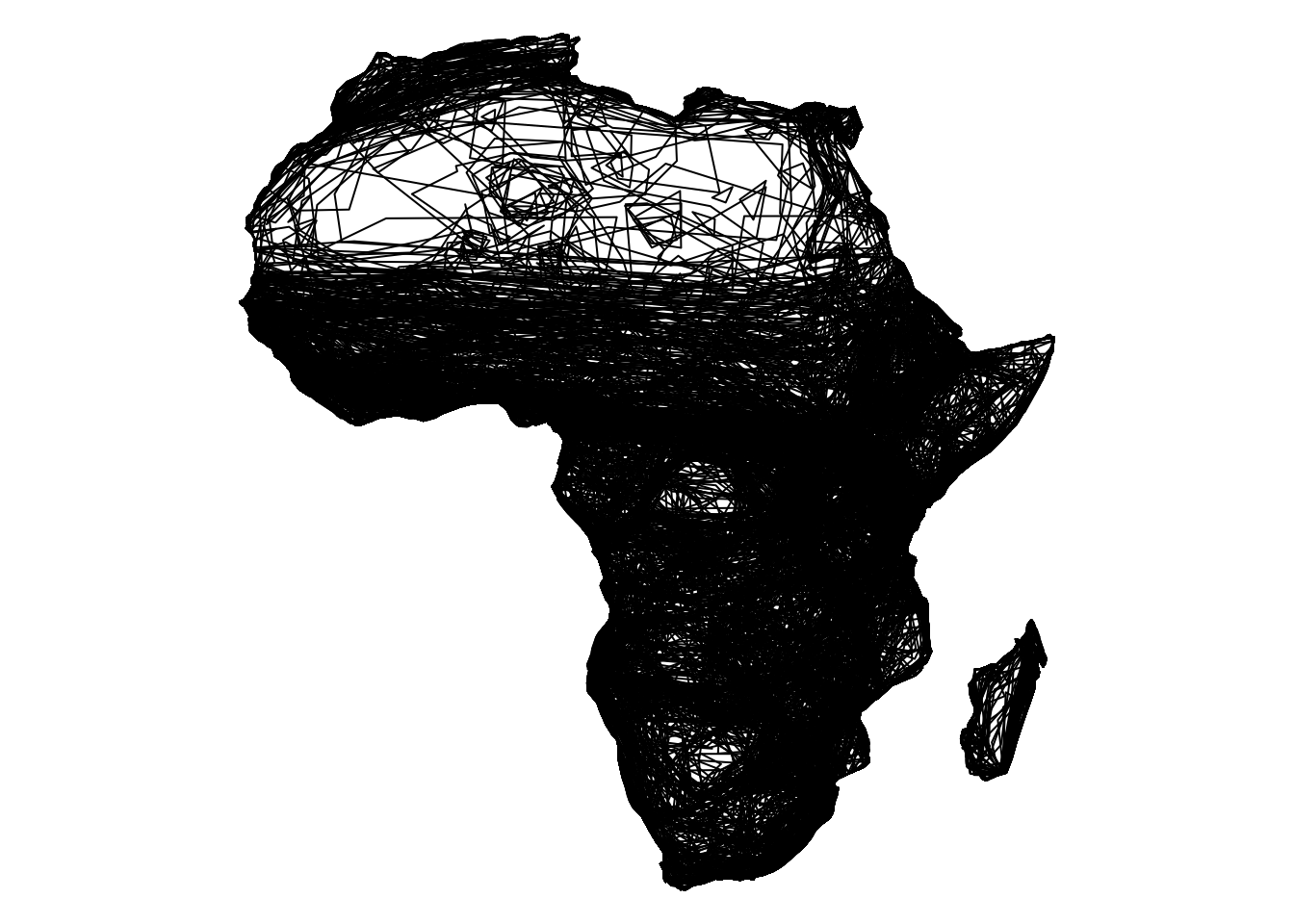
With st_intersection(), only the portion of population ranges within Africa are kept. Then, ranges are ‘summarized’ by species, which means that for species with several rows in the data frame, these rows are combined into one row with a (multi) polygon describing the entire range of this species. The use of dplyr::group_by() in combination with dplyr::summarize() with an sf object is another great example for the integration of the tidyverse functionality in the sf package.

africa_mammals <- st_intersection(mammals, africa_map) %>% 
  group_by(binomial) %>% 
  summarize()
{
  par(mar = c(0, 0, 0, 0))
  plot(st_geometry(africa_mammals))
}

4.2 Combine ranges with the grid

The range polygons can be combined with the grid map using the sf::st_join() function. Then, the number of species is counted per grid cell using the grid_id column created above.

# This may take a few minutes
species_per_cell <- africa_grid_clipped %>% 
  st_join(africa_mammals)

species_per_cell_sums <- species_per_cell %>% 
  group_by(grid_id) %>% 
  summarize(species_n = n())

4.3 Create the plot

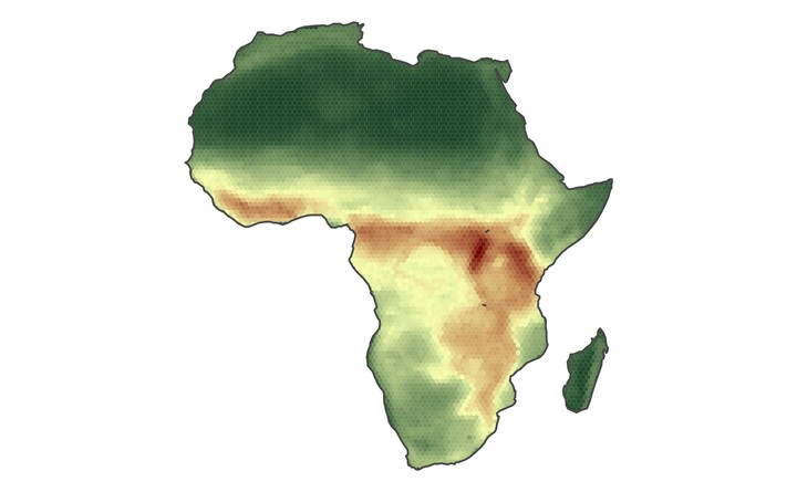
The standard output with plot() looks like this.

plot(species_per_cell_sums["species_n"])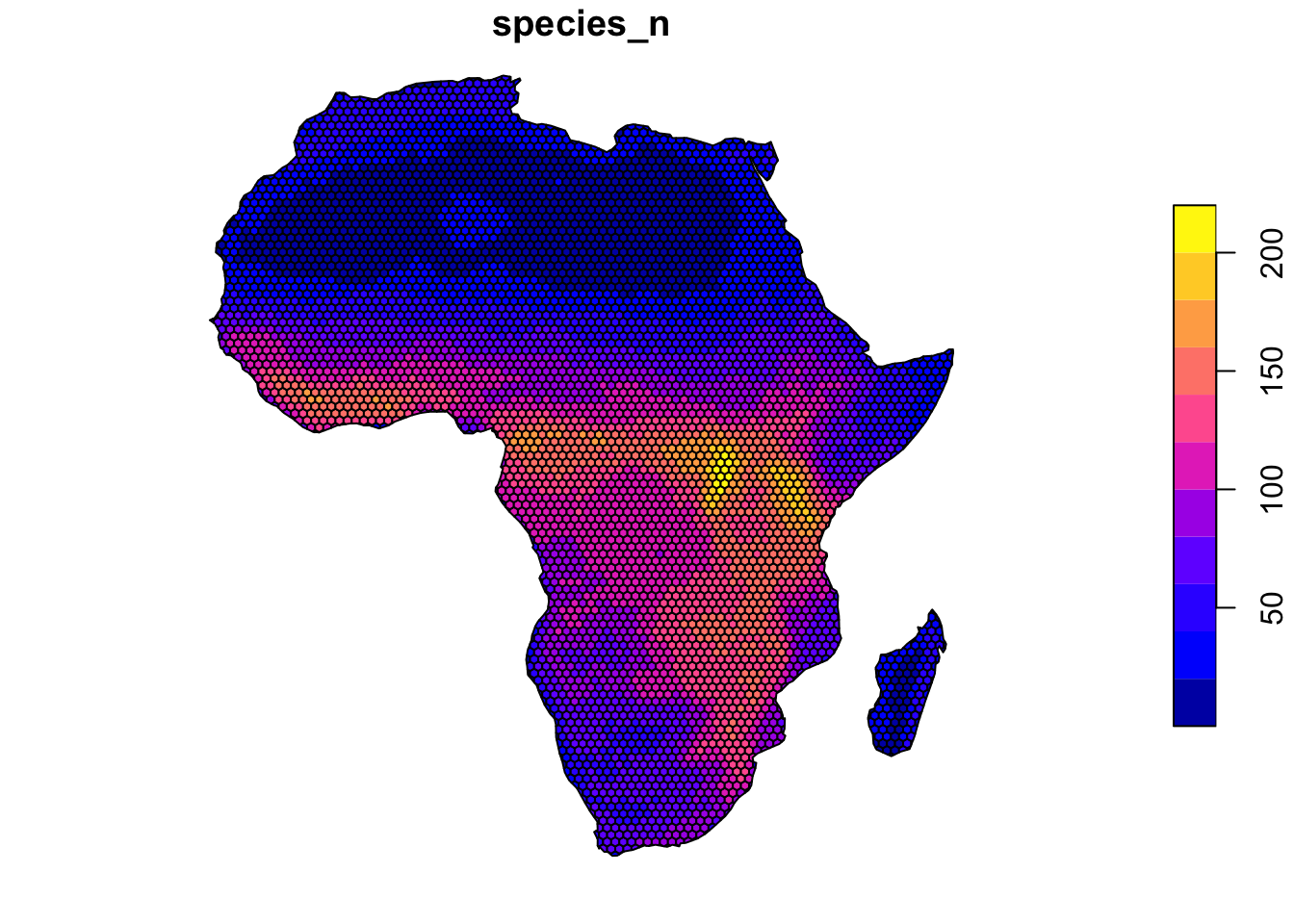

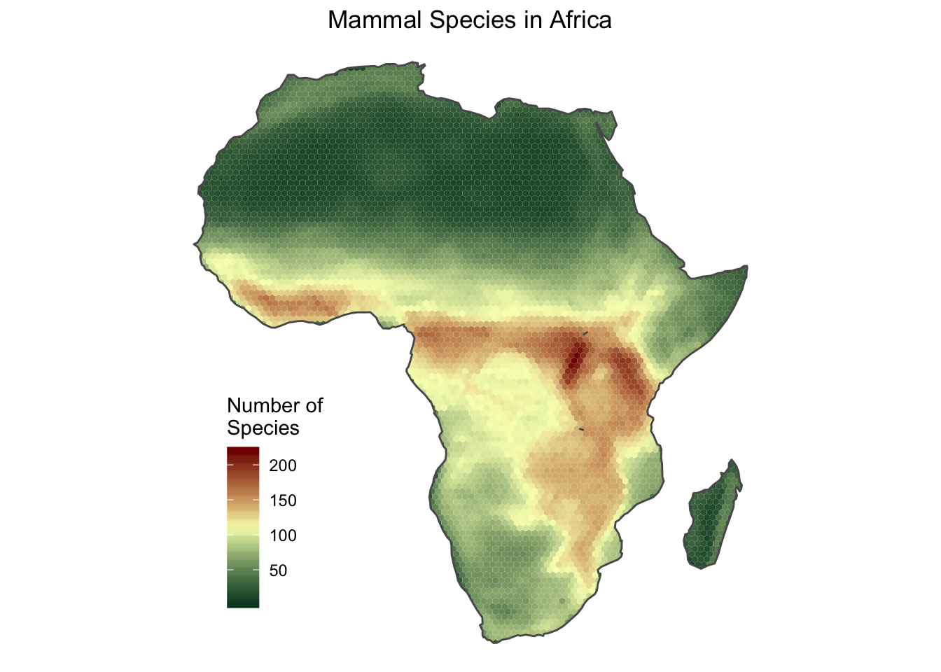
The plot created with plot() can be customized, but I find it easier to customize plots with the ggplot2 package. Therefore, I create another plot with ggplot() using a different color palette, and applying some other modifications.

african_mammals_map <- ggplot() +
  geom_sf(data = species_per_cell_sums,
          aes(fill = species_n),
          size = 0) +
  scale_fill_gradient2(name = "Number of\nSpecies",
                       low = "#004529",
                       mid = "#f7fcb9",
                       high = "#7f0000",
                       midpoint = max(species_per_cell_sums$species_n)/2) +
  geom_sf(data = africa_map, fill = NA) +
  labs(title = "Mammal Species in Africa") +
  theme_void() +
  theme(legend.position = c(0.1, 0.1),
        legend.justification = c(0, 0),
        plot.title = element_text(hjust = .5))
african_mammals_map