Creation and Detection of Clusters in Social Networks - Part 1

Last updated on Jan 3, 2020 7 min read 0 Comments

Social networks often exhibit some kind of clustering (or community structure), such as distinct social groups in animal societies, or kin groups (or families) within social groups. Individuals within such clusters are more likely to interact with each other than individuals from different clusters.

There are many algorithms to detect clusters in social networks, and one might work better than another under some circumstances (see, e.g., Emmons et al. 2016). Therefore, the aim of this and the next post is to simulate clustered social networks, and then to apply and compare some of the methods provided by the R-package igraph with these networks.

Note that there are functions available for R to create such networks, but here I create these networks ‘from scratch’ for two reasons:

It is easier to understand (and modify) the process underlying the network simulation.
Some clusters might be ‘closer’ to each other than other clusters. For example, individuals from two close families might be more likely to interact with each other than with individuals from other families. Perhaps, this can be achieved with the available functions, but I preferred to model these different degrees of clustering on my own.

This project will consist of two parts:

1. Simulate clustered social networks. I will simulate values of an ‘association index’ (reflecting social relationships) for dyads of individuals within the same groups, for dyads of individuals from ‘close’ groups, and for dyads consisting of individuals from different groups that are not close to each other. In total, I will simulate four different scenarios with varying degrees of clustering.

2. Determine clustering using different methods and compare the results. I will use several of the methods provided by the igraph package to detect clusters in these simulated networks. Then, I will calculate and compare the modularity of different networks, the number of detected clusters in comparison to simulated clusters, and the proportion of dyads correctly assigned to the same cluster.

1. Simulate clustered social networks

1.1 Prepare R

rm(list = ls())
library(tidyverse)
library(tidygraph)
library(ggraph)
library(igraph)

1.2 Create a dataframe with identities and group memberships of individuals

# Specify number of individuals and groups (or clusters)
n_inds <- 50
n_groups <- 4

# Create IDs for all individuals and assign random social groups to individuals
set.seed(1209)
individual_df <- tibble(
  Ind = paste0("ind_", str_pad(1:n_inds, width = nchar(n_inds), pad = "0")),
  Group = sample(x = paste0("group_", letters[1:n_groups]),
                 size = n_inds,
                 replace = T))

# Create a dataframe with all possible combinations of individuals except 'self-relationships'
network_df <- expand.grid(Ind_A = individual_df$Ind,
                          Ind_B = individual_df$Ind,
                          stringsAsFactors = F) %>%
  left_join(select(individual_df, Ind_A = Ind, Ind_A_Group = Group),
            by = "Ind_A") %>% 
  left_join(select(individual_df, Ind_B = Ind, Ind_B_Group = Group),
            by = "Ind_B") %>% 
  filter(Ind_A != Ind_B)

# Limit the dataframe to one row per dyad for an undirected network
network_df <- network_df %>% 
  arrange(Ind_A, Ind_B) %>% 
  mutate(dyad = if_else(Ind_A < Ind_B, paste0(Ind_A, "_", Ind_B),
                        paste0(Ind_B, "_", Ind_A))) %>% 
  distinct(dyad, .keep_all = T)

head(network_df)

##    Ind_A  Ind_B Ind_A_Group Ind_B_Group          dyad
## 1 ind_01 ind_02     group_b     group_a ind_01_ind_02
## 2 ind_01 ind_03     group_b     group_c ind_01_ind_03
## 3 ind_01 ind_04     group_b     group_b ind_01_ind_04
## 4 ind_01 ind_05     group_b     group_d ind_01_ind_05
## 5 ind_01 ind_06     group_b     group_a ind_01_ind_06
## 6 ind_01 ind_07     group_b     group_b ind_01_ind_07

1.3 Assign values (or ‘weights’) to all dyadic relationships.

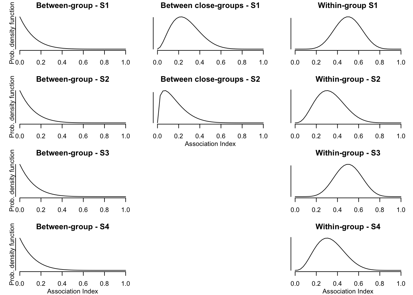
Here, I use 4 different scenarios:

1. Scenario (S1): Within-group relationships (wgr) are relatively strong in comparison to between-group relationships (bgr). Relationships of individuals between ‘close groups’ (bcgr) are intermediate.
2. Scenario (S2): Similar to S1, but differences between wgr, bcgr, and bgr are smaller.
3. Scenario (S3): Wgr are relatively strong in comparison to bgr. This scenario is identical to S1 except that there are no close groups.
4. Scenario (S4): Differences between wgr and bgr are smaller than in S3. This scenario is identical to S2 except that there are no close groups.

Thus, bgr are the same in all four scenarios, only bcgr and wgr are varied. Furthermore, wgr are the same for S1 and S3, and for S2 and S4 (see plot below).

To create the social networks, I sample values from beta distributions simulating an Association Index. Such an index is commonly used in animal behavioural research to assess relationships between individuals (see, e.g., the great book by Whitehead, 2008), and they range from 0 to 1. For example, individuals that never associate with each other would have an association index of 0, and two individuals that are always associated with each other have an index of 1.

# Set the parameters (i.e. shape parameters of the beta distribution) for all 4
# scenarios
bgr <- c(1, 8)
bcgr_1 <- c(3, 8)
wgr_1 <- wgr_3 <- c(8, 8)

bcgr_2 <- c(1.5, 8)
wgr_2 <- wgr_4 <- c(4, 8)

# Define function for plotting of beta distributions
plot_beta <- function(x, alpha_beta, main = "", xlab = "", ylab = "", ...){
  alpha = alpha_beta[1]
  beta =  alpha_beta[2]
  plot(x, dbeta(x, alpha, beta), type = "l",
       yaxt = "n", xlab = "", ylab = "", bty = "n", ...)
  title(ylab = ylab, line = 0)
  title(xlab = xlab, line = 2)
  title(main = main, line = 1)
  axis(side = 2, label = F, lwd.ticks = F)
}
# Plot the distributions of social relationships according to these parameters
{
  par(mfrow = c(4,3), mar = c(3, 2, 2, 1))
  x <- seq(0, 1, length.out = 40)
  
  # S1
  plot_beta(x, bgr, main = "Between-group - S1",
            ylab = "Prob. density function")
  plot_beta(x, bcgr_1, main = "Between close-groups - S1")
  plot_beta(x, wgr_1, main = "Within-group S1")
  
  # S2
  plot_beta(x, bgr, main = "Between-group - S2",
            ylab = "Prob. density function")
  plot_beta(x, bcgr_2, main = "Between close-groups - S2",
            xlab = "Association Index")
  plot_beta(x, wgr_2, main = "Within-group - S2")
  
  # S3
  plot_beta(x, bgr, main = "Between-group - S3",
            ylab = "Prob. density function")
  plot.new()
  plot_beta(x, wgr_3, main = "Within-group - S3")
  
  # S4
  plot_beta(x, bgr, main = "Between-group - S4", 
            ylab = "Prob. density function",
            xlab = "Association Index")
  plot.new()
  plot_beta(x, wgr_4, main = "Within-group - S4",
            xlab = "Association Index")
  
}

These distributions can be used to get values for the strength of relationships. To do so, I first define a function to sample dyadic values from the different distributions depending on group membership of both individuals. Then, I use this function to get values for all dyads and for all scenarios. For S1 and S2, group A and B are defined as the close groups.

get_weights <- function(network_df, wgr, bgr, bcgr = NA, close_groups = NA){
  # Create empty vector for all weights
  weights = rep(NA_real_, time = nrow(network_df))
  # Go through all dyads and sample from respective distribution, dependent on
  # the group membership of both individuals
  for(i in seq_along(weights)){
    ind_A_group <- network_df[i, "Ind_A_Group"]
    ind_B_group <- network_df[i, "Ind_B_Group"]
    # Both individuals in same group
    if(ind_A_group == ind_B_group){
      weights[i] <- rbeta(n = 1, shape1 = wgr[1], shape2 = wgr[2])
    }
    # Individuals in different groups
    if(ind_A_group != ind_B_group){
      weights[i] <- rbeta(n = 1, shape1 = bgr[1], shape2 = bgr[2])
    }
    # If some groups are 'closer' to each other, use specified distributions for
    # this kind of relationships
    if(all(!is.na(bcgr)) & all(!is.na(close_groups)) &
       ind_A_group != ind_B_group &
       ind_A_group %in% close_groups & 
       ind_B_group %in% close_groups){
      weights[i] <- rbeta(n = 1, shape1 = bcgr[1], shape2 = bcgr[2])
      }
  }
  return(weights)
}

set.seed(1209)
network_df$S1 <- get_weights(network_df, wgr = wgr_1, bgr = bgr, bcgr = bcgr_1,
                             close_groups = c("group_a", "group_b"))
network_df$S2 <- get_weights(network_df, wgr = wgr_2, bgr = bgr, bcgr = bcgr_2,
                             close_groups = c("group_a", "group_b"))
network_df$S3 <- get_weights(network_df, wgr = wgr_3, bgr = bgr)
network_df$S4 <- get_weights(network_df, wgr = wgr_4, bgr = bgr)

As the last step for part 1 of this post, I will illustrate the created networks using the ggraph package (look here for an introduction to this package by the author)

set.seed(1209)
clustered_network_plot <- network_df %>% 
  pivot_longer(cols = matches("S\\d"),
               names_to = "Scenario",
               values_to = "weight") %>% 
  select(from = Ind_A, to = Ind_B, weight, Scenario) %>% 
  filter(weight >= 0.3) %>% 
  as_tbl_graph() %>% 
  activate(nodes) %>% 
  left_join(distinct(individual_df, name = Ind, group = Group),
            by = "name") %>% 
  ggraph(., layout = "fr") +
  geom_edge_arc(aes(width = weight),
                alpha = 0.4, strength = 0.1) +
  scale_edge_width(name = "Association Index",
                   range = c(0.2, 1)) +
  geom_node_point(aes(fill = group, shape = group),
                  size = 2) +
  scale_fill_brewer(type = "qual", palette = 2) +
  scale_shape_manual(values = c(21, 22, 23, 24)) +
  facet_edges(~Scenario) +
  theme_graph()

clustered_network_plot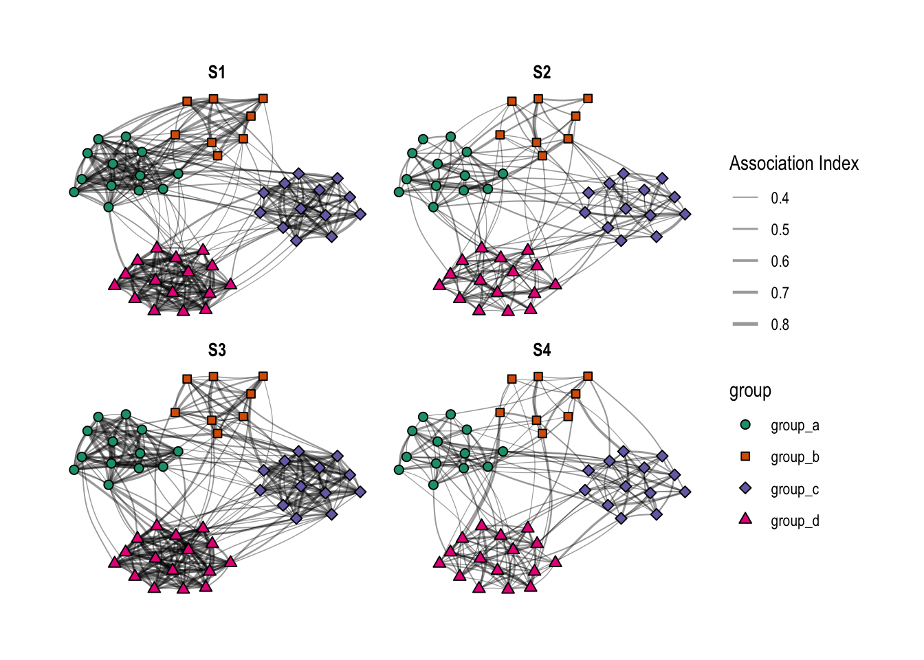

As modeled above, S1 and S3 are very similar, except that group A and B are closer to each other in S1. S2 and S4 have both weaker within-group relationships compared to their counterparts S1 and S3, respectively. Thus, I have four different networks with different degrees of clustering, and in two of these networks, two of the four groups are closer to each other than to the other groups.

In the next post, I will use different algorithms from the igraph package to check how well these clusters can be detected.

Creation and Detection of Clusters in Social Networks - Part 1

1. Simulate clustered social networks

1.1 Prepare R

1.2 Create a dataframe with identities and group memberships of individuals

1.3 Assign values (or ‘weights’) to all dyadic relationships.

Urs Kalbitzer