Creation and Detection of Clusters in Social Networks - Part 2

In the previous post, I simulated clustered networks with varying strength of within-group, between-close-groups, and between-group social relationships. In part 2, I am using some of the methods provided by the igraph package to test how well these simulated clusters can be (re)-detected.
2. Determine clustering using different methods and compare the results
2.1 Prepare R
rm(list = ls())
library(tidyverse)
library(tidygraph)
library(ggraph)
library(igraph)
In addition to these packages, this notebook requires the installation of the following packages: DT, cowplot, ggrepel.
2.2 Recreate the network from previous post
To avoid repetition, the code is not shown here, but can be copied from the previous post. The two objects that are required from there are individual_df and network_df.
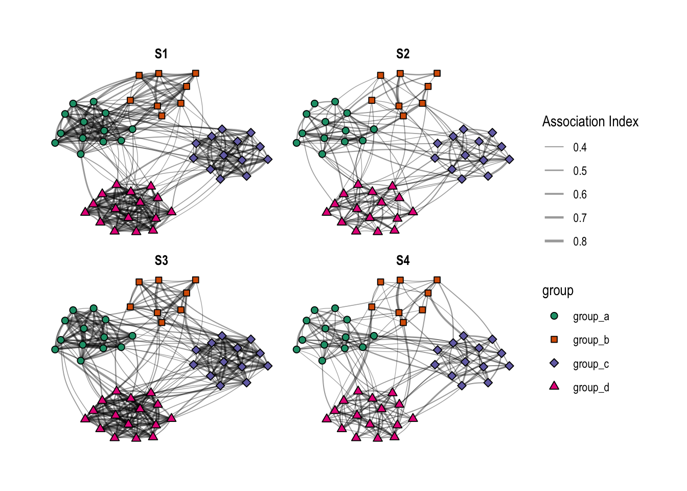
The networks looked like that:

One important note: My motivation for this small project was my research on a group of ~50 adult red colobus monkeys. Therefore, I simulated networks where most individuals were somehow connected. The plot above, however, only shows association indices \(\ge\) 0.3 to make it easier to see the clusters. The complete network is much denser (see the final plot of this post). After finalizing the draft of this post, I realized that this may have affected how well (or not) the algorithms detected the (sub)-groups and therefore wanted to mention it here.
2.3 Use different algorithms to detect clusters
The igraph-package provides several functions to detect communities within a network, which start with cluster_ (type ?communities in R for a complete list). Most of these algorithms are explained here and here.
Before using the cluster_ functions, the networks have to be transformed into igraph objects.
df_to_network <- function(network_df, weight_col){
  network <- graph_from_data_frame(select(network_df,
                                          from = Ind_A, to = Ind_B,
                                          weight = matches(weight_col)),
                              directed = FALSE)
  return(network)
}

network_1 <- df_to_network(network_df, weight_col = "S1")
network_2 <- df_to_network(network_df, weight_col = "S2")
network_3 <- df_to_network(network_df, weight_col = "S3")
network_4 <- df_to_network(network_df, weight_col = "S4")
Here’s the standard output for such an object:
network_1## IGRAPH 1485755 UNW- 50 1225 --
## + attr: name (v/c), weight (e/n)
## + edges from 1485755 (vertex names):
## [1] ind_01--ind_02 ind_01--ind_03 ind_01--ind_04 ind_01--ind_05 ind_01--ind_06
## [6] ind_01--ind_07 ind_01--ind_08 ind_01--ind_09 ind_01--ind_10 ind_01--ind_11
## [11] ind_01--ind_12 ind_01--ind_13 ind_01--ind_14 ind_01--ind_15 ind_01--ind_16
## [16] ind_01--ind_17 ind_01--ind_18 ind_01--ind_19 ind_01--ind_20 ind_01--ind_21
## [21] ind_01--ind_22 ind_01--ind_23 ind_01--ind_24 ind_01--ind_25 ind_01--ind_26
## [26] ind_01--ind_27 ind_01--ind_28 ind_01--ind_29 ind_01--ind_30 ind_01--ind_31
## [31] ind_01--ind_32 ind_01--ind_33 ind_01--ind_34 ind_01--ind_35 ind_01--ind_36
## [36] ind_01--ind_37 ind_01--ind_38 ind_01--ind_39 ind_01--ind_40 ind_01--ind_41
## + ... omitted several edgesAnd here’s the output if one of the cluster_ functions is applied to a network, in this example the fast-greedy algorithm to the first network (S1):
cluster_fast_greedy(network_1)## IGRAPH clustering fast greedy, groups: 3, mod: 0.32
## + groups:
## $`1`
## [1] "ind_05" "ind_09" "ind_12" "ind_17" "ind_20" "ind_23" "ind_26" "ind_29"
## [9] "ind_31" "ind_32" "ind_36" "ind_38" "ind_40" "ind_43" "ind_49" "ind_50"
##
## $`2`
## [1] "ind_03" "ind_15" "ind_19" "ind_21" "ind_22" "ind_27" "ind_28" "ind_37"
## [9] "ind_39" "ind_45" "ind_46" "ind_47" "ind_48"
##
## $`3`
## [1] "ind_01" "ind_02" "ind_04" "ind_06" "ind_07" "ind_08" "ind_10" "ind_11"
## + ... omitted several groups/verticesThus, the function tries to detect clusters (called groups) and assigns each individual to such a group. Furthermore, it calculates modularity (mod).
The aim of this post is to use several of these functions and then compare 1) the number of detected groups and 2) the detected group membership of all individuals to what was simulated (i.e., the ‘true’ values). Furthermore, I will extract the global modularity, which can be used to compare the quality of different cluster methods (many of the algorithms try to maximize modularity when searching for clusters).
Therefore, I first define a function to apply the specified algorithm to a network, extract these metrics from the resulting communities-object, and return them in a dataframe.
get_communities <- function(igraph_network, cluster_method = NULL){
  if(is.null(cluster_method)) { stop("no method specificied") }
  community_object <- do.call(cluster_method, list(igraph_network))
  return(tibble(Ind = community_object$names,
                Ind_Cluster = community_object$membership,
                global_modularity = modularity(igraph_network,
                                               community_object$membership,
                                               weights = E(igraph_network)$weight),
                method = cluster_method) %>%
           arrange(Ind))
}
Example:
get_communities(network_1, "cluster_fast_greedy")## # A tibble: 50 x 4
## Ind Ind_Cluster global_modularity method
## <chr> <dbl> <dbl> <chr>
## 1 ind_01 3 0.318 cluster_fast_greedy
## 2 ind_02 3 0.318 cluster_fast_greedy
## 3 ind_03 2 0.318 cluster_fast_greedy
## 4 ind_04 3 0.318 cluster_fast_greedy
## 5 ind_05 1 0.318 cluster_fast_greedy
## 6 ind_06 3 0.318 cluster_fast_greedy
## 7 ind_07 3 0.318 cluster_fast_greedy
## 8 ind_08 3 0.318 cluster_fast_greedy
## 9 ind_09 1 0.318 cluster_fast_greedy
## 10 ind_10 3 0.318 cluster_fast_greedy
## # … with 40 more rowsUsing this function, I apply several of the provided igraph methods with the four networks.
networks <- grep("network_\\d", ls(), value = T)
cluster_methods <- c("cluster_fast_greedy", "cluster_infomap",
                     "cluster_label_prop", "cluster_optimal",
                     "cluster_louvain", "cluster_walktrap")

for(network_i in seq_along(networks)){
  for(cluster_method_j in seq_along(cluster_methods)){
    df_temp <- get_communities(igraph_network = get(networks[[network_i]]),
                               cluster_method = cluster_methods[[cluster_method_j]])
    df_temp$network <- networks[[network_i]]
    if(network_i == 1 & cluster_method_j == 1) community_df <- df_temp
    else community_df <- bind_rows(community_df, df_temp)
  }
}

# Show structure of created dataframe
str(community_df)
## Classes 'tbl_df', 'tbl' and 'data.frame': 1200 obs. of 5 variables:
## $ Ind : chr "ind_01" "ind_02" "ind_03" "ind_04" ...
## $ Ind_Cluster : num 3 3 2 3 1 3 3 3 1 3 ...
## $ global_modularity: num 0.318 0.318 0.318 0.318 0.318 ...
## $ method : chr "cluster_fast_greedy" "cluster_fast_greedy" "cluster_fast_greedy" "cluster_fast_greedy" ...
## $ network : chr "network_1" "network_1" "network_1" "network_1" ...The resulting table includes the global modularity for each method and network, and the estimated group membership ($Ind_Cluster) of all individuals within each networks using each of the methods.
2.4 Compare the detected clusters with simulated groups
Finally, I compare the results of the different algorithms with the simulated networks.
# Set up dataframe for loop
cluster_summary <- tibble(
  Cluster_method = rep(cluster_methods, each = length(networks)),
  Scenario = rep(networks, times = length(cluster_methods)),
  Dyads_n = length(unique(network_df$dyad)),
  Groups_n = length(unique(network_df$Ind_A_Group)),
  Clusters_n = NA,
  Dyads_correct_n = NA,
  Dyads_correct_prop = NA,
  Modularity = NA)

# Use a loop to summarize for all methods and networks the 1) number of clusters
# in comparison to simulated groups, and 2) the number of dyads correctly placed
# together in a cluster.
for(row_i in 1:nrow(cluster_summary)){
  community_temp <- filter(community_df,
                           method == cluster_summary[row_i,]$Cluster_method &
                           network == cluster_summary[row_i,]$Scenario)

  cluster_summary_temp <- network_df %>%
    select(Ind_A, Ind_B, Ind_A_Group, Ind_B_Group) %>%
    left_join(select(community_temp, Ind_A = Ind, Ind_A_Cluster = Ind_Cluster),
              by = "Ind_A") %>%
    left_join(select(community_temp, Ind_B = Ind, Ind_B_Cluster = Ind_Cluster),
              by = "Ind_B") %>%
    mutate(same_group = (Ind_A_Group == Ind_B_Group),
           same_cluster = (Ind_A_Cluster == Ind_B_Cluster))

    cluster_summary[row_i,]$Clusters_n = length(unique(community_temp$Ind_Cluster))
    cluster_summary[row_i,]$Dyads_correct_n = sum(cluster_summary_temp$same_group == cluster_summary_temp$same_cluster)
    cluster_summary[row_i,]$Modularity = unique(community_temp$global_modularity)
}

# Calculate variables comparing simulated with detected clusters and apply some
# other cosmetic changes
cluster_summary <- cluster_summary %>%
  mutate(Dyads_correct_prop = Dyads_correct_n/Dyads_n,
         Clusters_vs_Groups = Clusters_n/Groups_n,
         Scenario = str_replace(Scenario, "network_", "S"),
         Cluster_method = str_remove(Cluster_method, "cluster_")) %>%
  mutate_if(is.numeric, ~round(., 2))
This is the resulting table:
knitr::kable(cluster_summary)| Cluster_method | Scenario | Dyads_n | Groups_n | Clusters_n | Dyads_correct_n | Dyads_correct_prop | Modularity | Clusters_vs_Groups |
|---|---|---|---|---|---|---|---|---|
| fast_greedy | S1 | 1225 | 4 | 3 | 1121 | 0.92 | 0.32 | 0.75 |
| fast_greedy | S2 | 1225 | 4 | 3 | 1121 | 0.92 | 0.22 | 0.75 |
| fast_greedy | S3 | 1225 | 4 | 4 | 1225 | 1.00 | 0.31 | 1.00 |
| fast_greedy | S4 | 1225 | 4 | 3 | 1121 | 0.92 | 0.22 | 0.75 |
| infomap | S1 | 1225 | 4 | 3 | 1121 | 0.92 | 0.32 | 0.75 |
| infomap | S2 | 1225 | 4 | 1 | 304 | 0.25 | 0.00 | 0.25 |
| infomap | S3 | 1225 | 4 | 1 | 304 | 0.25 | 0.00 | 0.25 |
| infomap | S4 | 1225 | 4 | 1 | 304 | 0.25 | 0.00 | 0.25 |
| label_prop | S1 | 1225 | 4 | 2 | 848 | 0.69 | 0.23 | 0.50 |
| label_prop | S2 | 1225 | 4 | 1 | 304 | 0.25 | 0.00 | 0.25 |
| label_prop | S3 | 1225 | 4 | 3 | 1121 | 0.92 | 0.29 | 0.75 |
| label_prop | S4 | 1225 | 4 | 2 | 848 | 0.69 | 0.17 | 0.50 |
| optimal | S1 | 1225 | 4 | 3 | 1121 | 0.92 | 0.32 | 0.75 |
| optimal | S2 | 1225 | 4 | 3 | 1121 | 0.92 | 0.22 | 0.75 |
| optimal | S3 | 1225 | 4 | 4 | 1225 | 1.00 | 0.31 | 1.00 |
| optimal | S4 | 1225 | 4 | 4 | 1225 | 1.00 | 0.23 | 1.00 |
| louvain | S1 | 1225 | 4 | 3 | 1121 | 0.92 | 0.32 | 0.75 |
| louvain | S2 | 1225 | 4 | 3 | 1121 | 0.92 | 0.22 | 0.75 |
| louvain | S3 | 1225 | 4 | 4 | 1225 | 1.00 | 0.31 | 1.00 |
| louvain | S4 | 1225 | 4 | 4 | 1225 | 1.00 | 0.23 | 1.00 |
| walktrap | S1 | 1225 | 4 | 3 | 1121 | 0.92 | 0.32 | 0.75 |
| walktrap | S2 | 1225 | 4 | 3 | 1121 | 0.92 | 0.22 | 0.75 |
| walktrap | S3 | 1225 | 4 | 4 | 1225 | 1.00 | 0.31 | 1.00 |
| walktrap | S4 | 1225 | 4 | 4 | 1225 | 1.00 | 0.23 | 1.00 |
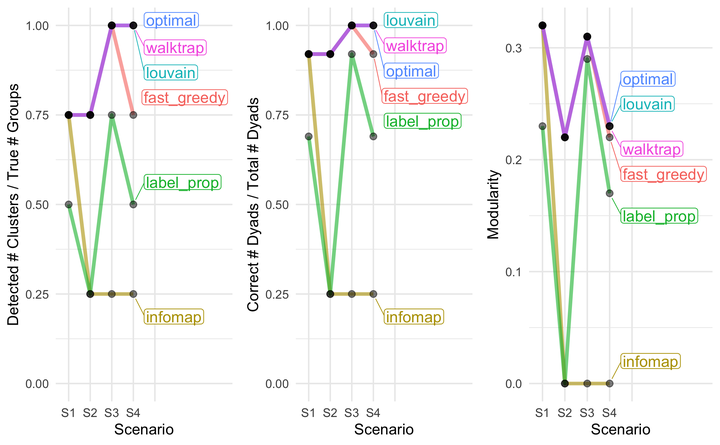
Perhaps, it’s a bit easier to interpret the results when graphically illustrated.
2.5 Illustrate results
create_plot <- function(df, y_var, y_title){
  y_var <- sym(y_var)
  ggplot(data = df,
            aes(x = Scenario, y = !!y_var, group = Cluster_method, color = Cluster_method)) +
  geom_line(size = 1.25, alpha = .6) +
  geom_point(color = "black", size = 2, alpha = .5) +
  ggrepel::geom_label_repel(data = filter(df, Scenario == "S4"),
            aes(x = Scenario, y = !!y_var, color = Cluster_method, label = Cluster_method),
            size = 4,
            hjust = 0, nudge_x = .5, direction = "y",
            label.padding = .1, point.padding = .5, segment.size = .25,
            show.legend = F) +
  scale_x_discrete(limits = c("S1", "S2", "S3", "S4", rep("", 4))) +
  scale_y_continuous(name = y_title, limits = c(0, NA)) +
  theme_minimal() +
  theme(legend.position = "none")
}

cluster_plot <- create_plot(df = cluster_summary,
                            y_var = "Clusters_vs_Groups",
                            y_title = "Detected # Clusters / True # Groups")
dyad_plot <- create_plot(df = cluster_summary,
                         y_var = "Dyads_correct_prop",
                         y_title = "Correct # Dyads / Total # Dyads")
modularity_plot <- create_plot(df = cluster_summary,
                               y_var = "Modularity",
                               y_title = "Modularity")

cowplot::plot_grid(cluster_plot, dyad_plot, modularity_plot, ncol = 3)
2.6 Conclusions
For the created networks, here are my conclusions:
- None(!) of the tested algorithms correctly identified the number of groups in S1 and S2 (the two scenarios with ‘close groups’). But three of the four algorithms that did best in these two scenarios (louvain, walktrap, optimal) perfectly identified groups in S3 and S4. Thus, under the circumstances simulated in S1 and S2, which are fairly common in reality I believe, one should be careful with the interpretation of the number of detected clusters.
- With the exception of S1, the infomap algorithm did not very well and put all individuals in the same cluster. The label_prob method was a bit better than infomap, but always failed to identify the correct number of groups.
- The comparison of modularity values confirms that the algorithms with the highest modularity values also were the best in identifying groups and individual group memberships (note that these modularity values are calculated without knowing the ‘true’ groups).
- As mentioned above and shown in the plot below, the simulation actually created many, fairly weak relationships among individuals, even among individuals from different groups. Perhaps, this makes the detection of clusters challenging for the algorithms, especially if the distinction between different groups within a larger community is variable (as in S1, S2). Thus, when applying such methods to identify clusters, it seems to be important to simulate some networks similar to the observed networks and try which methods are most appropriate given the circumstances.
2.7 Identifying and illustrating clusters with ggraph
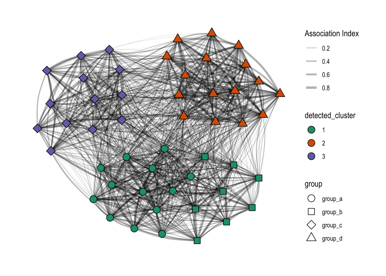
The ggraph package also supports the use of the igraph::cluster_ functions, which can be nicely used for a quick look at clusters. Here, both the detected clusters (using different colors) and the simulated groups (using different shapes) are shown. In contrast to the plots above, all relationships (or edges) are shown, including those < 0.3, which makes the networks look much denser than in the other plots.
network_df %>%
  select(from = Ind_A, to = Ind_B, weight = S1) %>%
  as_tbl_graph(directed = FALSE) %>%
  activate(nodes) %>%
  left_join(distinct(individual_df, name = Ind, group = Group),
            by = "name") %>%
  mutate(detected_cluster = as.factor(group_louvain())) %>%
  ggraph(., layout = "fr") +
  geom_edge_arc(aes(width = weight),
                alpha = 0.3, strength = 0.1) +
  scale_edge_width(name = "Association Index", range = c(0, 1.5)) +
  geom_node_point(aes(fill = detected_cluster, shape = group),
                  color = "black", size = 4) +
  scale_fill_brewer(type = "qual", palette = 2) +
  scale_shape_manual(values = c(21, 22, 23, 24)) +
  theme_graph() +
  guides(fill = guide_legend(override.aes = list(shape=21)))
It’s clear from this plot that group_a and group_b are put in the same cluster by the louvain method.